
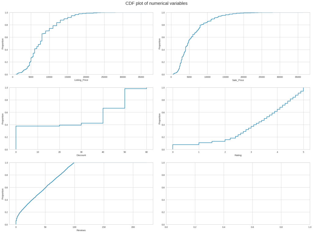
The provided code below generates a grid of subplots (dynamic rows and 2 columns) and plots cumulative distribution function (CDF) plots for numerical variables in a DataFrame (df).
num_col = df.select_dtypes(include=np.number).columns.to_list()
col_count = len(num_col)

fig_rows = (col_count // 2 ) + 1 if col_count % 2 != 0 else col_count //2

fig, axes = plt.subplots(fig_rows, 2, figsize=(20, 15))
fig.suptitle("CDF plot of numerical variables", fontsize=20)
counter = 0
for i in range(fig_rows):
    sns.ecdfplot(ax=axes[i][0], x=df[num_col[counter]])
    counter = counter + 1
    if counter != col_count:
        sns.ecdfplot(ax=axes[i][1], x=df[num_col[counter]])
        counter = counter + 1
    else:
        pass

fig.tight_layout(pad=2.0)
GO ONE LEVEL DEEPER
How to read a CDF plot
A cumulative distribution function answers a practical question: what share of observations is less than or equal to a chosen value?
Choose a value
Start at the measurement you want to understand on the horizontal axis.
Meet the curve
Move upward until you reach the empirical CDF line.
Read the share
Move left to find the cumulative proportion on the vertical axis.
Keep in mind
- Steep sections indicate many observations in a narrow range.
- Horizontal gaps indicate ranges with few or no observations.
- Shared axes make distribution comparisons much easier.