
Calibration curves are specifically used for classification models. The primary goal of a calibration curve is to evaluate the reliability of the predicted probabilities in a classification task. A calibration curve checks how well predicted probabilities align with the actual observed frequencies (e.g., when a model predicts 70% probability of being positive, we expect about 70% of such instances to actually be positive).
In applications like medical diagnosis or risk assessment, you want the predicted probabilities to be accurate. For instance, if a model says there’s an 80% chance of a disease, you want that probability to reflect reality.
# Re-import necessary libraries after the code reset
import numpy as np
import matplotlib.pyplot as plt
from sklearn.datasets import make_classification
from sklearn.model_selection import train_test_split
from sklearn.naive_bayes import GaussianNB
from sklearn.linear_model import LogisticRegression
from sklearn.ensemble import RandomForestClassifier
from sklearn.svm import SVC
from sklearn.calibration import calibration_curve

# Create synthetic dataset for binary classification
X, y = make_classification(n_samples=1000, n_features=20, n_informative=10, n_redundant=5, random_state=42)
# n_informative = 10 means that 10 of out 20 features are useful and have impact on Y
# n_redundant= 5 means that 5 out of 20 features are linear combination of other features and add collinearity


# Split data into training and testing sets
X_train, X_test, y_train, y_test = train_test_split(X, y, test_size=0.3, random_state=42)

# Define classifiers
classifiers = {
    'Naive Bayes': GaussianNB(),
    'Logistic Regression': LogisticRegression(max_iter=1000),
    'Random Forest': RandomForestClassifier(n_estimators=100),
    'Support Vector Classifier': SVC(probability=True)
}

# Plot calibration curves
plt.figure(figsize=(10, 8))

# Loop through classifiers and plot calibration curves
for name, clf in classifiers.items():
    # Fit the classifier
    clf.fit(X_train, y_train)

    # Predict probabilities or decision function
    if hasattr(clf, "predict_proba"):
        y_prob = clf.predict_proba(X_test)[:, 1]
    else:
        y_prob = clf.decision_function(X_test)
        y_prob = (y_prob - y_prob.min()) / (y_prob.max() - y_prob.min())  # scale to [0, 1] for plotting

    # Calculate calibration curve
    fraction_of_positives, mean_predicted_value = calibration_curve(y_test, y_prob, n_bins=10)

    # Plot the calibration curve
    plt.plot(mean_predicted_value, fraction_of_positives, marker='o', linewidth=1, label=name)

# Plot a perfectly calibrated reference line
plt.plot([0, 1], [0, 1], linestyle='--', color='black', label='Perfectly Calibrated')

# Configure plot
plt.xlabel('Mean Predicted Probability')
plt.ylabel('Fraction of Positives')
plt.title('Calibration Curves (Reliability Plot)')
plt.legend()
plt.grid(True)
plt.show()
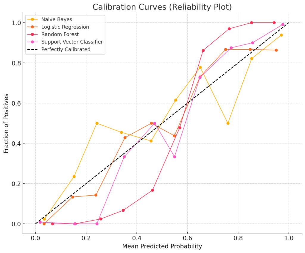
GO ONE LEVEL DEEPER
Calibration asks whether probabilities mean what they say
If predictions around 0.70 are well calibrated, roughly 70% of those cases should be positive. This is different from merely ranking positive cases above negative ones.
Near diagonal
Predicted probabilities closely match observed frequencies.
Below diagonal
The model is generally overconfident in the positive class.
Above diagonal
The model is generally underconfident in the positive class.
Keep in mind
- Use enough samples in each probability bin.
- Compare calibration together with discrimination metrics such as ROC-AUC.
- Calibrate on validation data, never on the final test set.